
Step-by-Step Guide to Building Excel Budget Templates for Tracking Revenue and Costs

Step-by-Step Guide to Building Excel Budget Templates for Tracking Revenue and Costs
Quick Links
- Create a Simple List
- Format the List as a Table
- Name the Table
- Add Totals for the Income and Expenses
- Summarize the Income and Expenses by Month
- Update the Income and Expenses PivotTables
Creating an expense and income spreadsheet can help you manage your personal finances. This can be a simple spreadsheet that provides an insight into your accounts and tracks your main expenses. Here’s how in Microsoft Excel.
Create a Simple List
In this example, we just want to store some key information about each expense and income. It doesn’t need to be too elaborate. Below is an example of a simple list with some sample data.
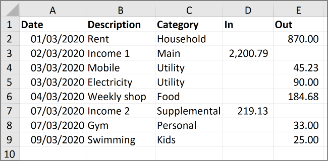
Enter column headers for the information you want to store about each expense and form of income along with several lines of data as shown above. Think about how you want to track this data and how you would refer to it.
This sample data is a guide. Enter the information in a way that is meaningful to you.
Format the List as a Table
Formatting the range as a table will make it easier to perform calculations and control the formatting.
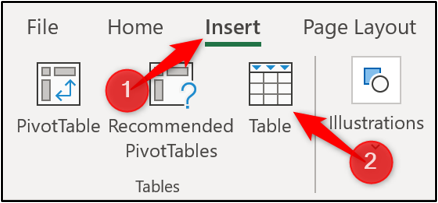
Click anywhere within your list of data and then select Insert > Table.
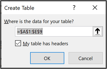
Highlight the range of data in your list that you want to use. Ensure that the range is correct in the “Create Table” window and that the “My Table Has Headers” box is checked. Click the “OK” button to create your table.
The list is now formatted as a table. The default blue formatting style will also be applied.
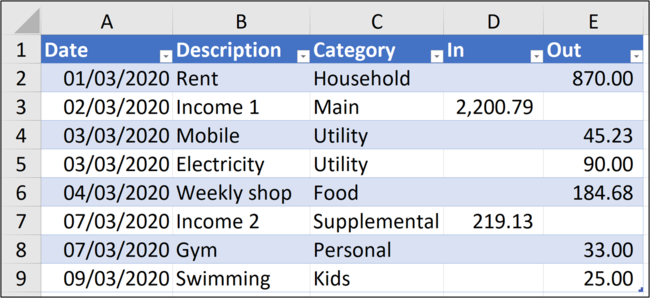
When more rows are added to the list, the table will automatically expand and apply formatting to the new rows.
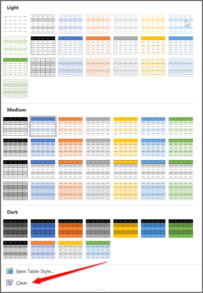
If you would like to change the table formatting style, select your table, click the “Table Design” button, and then the “More” button on the corner of the table styles gallery.

This will expand the gallery with a list of styles to choose from.
You can also create your own style or clear the current style by clicking the “Clear” button.
Name the Table
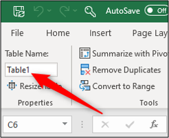
We will give the table a name to make it easier to refer to in formulas and other Excel features.
To do this, click in the table and then select the “Table Design” button. From there, enter a meaningful name such as “Accounts2020” into the Table Name box.
Add Totals for the Income and Expenses
Having your data formatted as a table makes it simple to add total rows for your income and expenses.
Click in the table, select “Table Design”, and then check the “Total Row” box.

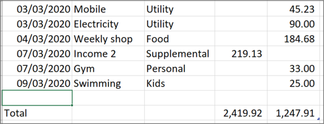
A total row is added to the bottom of the table. By default, it will perform a calculation on the last column.
In my table, the last column is the expense column, so those values are totaled.
Click the cell that you want to use to calculate your total in the income column, select the list arrow, and then choose the Sum calculation.
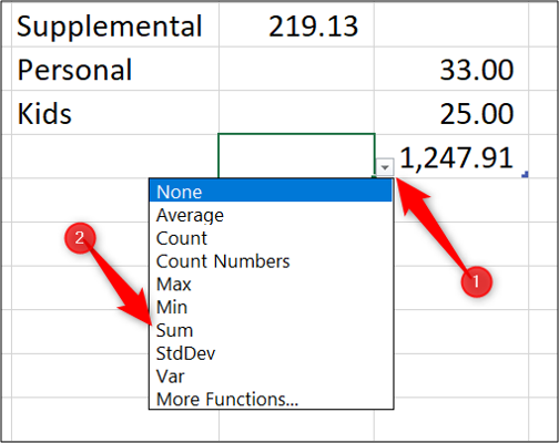
There are now totals for the income and the expenses.
When you have a new income or expense to add, click and drag the blue resize handle in the bottom-right corner of the table.
Drag it down the number of rows you want to add.
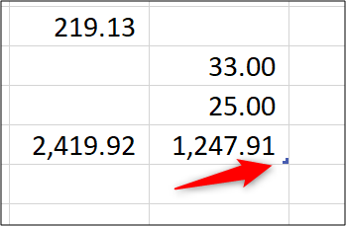
Enter the new data in the blank rows above the total row. The totals will automatically update.
Summarize the Income and Expenses by Month
It is important to keep totals of how much money is coming into your account and how much you are spending. However, it is more useful to see these totals grouped by month and to see how much you spend in different expense categories or on different types of expenses.
To find these answers, you can create a PivotTable.
Click in the table, select the “Table Design” tab, and then choose “Summarise With PivotTable”.

The Create PivotTable window will show the table as the data to use and will place the PivotTable on a new worksheet. Click the “OK” button.
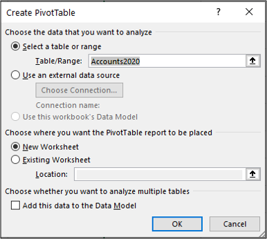
The PivotTable appears on the left, and a Field List appears on the right.
This is a quick demo to summarise your expense and income easily with a PivotTable. If you are new to PivotTables, check out this in-depth article .
To view a breakdown of your expense and income by month, drag the “Date” column into the “Rows” area and the “In” and “Out” columns into the “Values” area.
Be aware that your columns may be named differently.
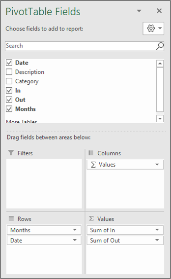
The “Date” field is automatically grouped into months. The “In” and “Out” fields are summed.
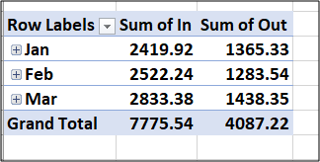
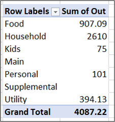
In a second PivotTable, you can view a summary of your expenses by category.
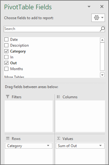
Click and drag the “Category” field into “Rows” and the “Out” field into “Values”.
The following PivotTable is created summarising expenses by category.
Update the Income and Expenses PivotTables
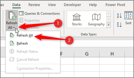
When new rows are added to the income and expenses table, select the “Data” tab, click the “Refresh All” arrow, and then choose “Refresh All” to update both PivotTables.
Also read:
- [Updated] 2024 Approved Unlock Earnings The Guide to Successful Vimeo Monetization
- [Updated] Enhance Engagement Sharing Videos on Instagram for 2024
- 2024 Approved Begin Your Journey Into Xp's Video Editing World
- 2024 Approved Real-Time Skype Monitoring with Live OBS Integration
- Activating the Virtual Keyboard on Your PC: Guidelines for Windows 11, 8 & 7
- How to Come up With the Best Pokemon Team On Samsung Galaxy M14 4G? | Dr.fone
- How to Successfully Repair a Nonfunctional ChatGPT App on Your iPhone Using These 9 Fixes
- Immediate Fixes for the Batman: Arkham Knight Fatal Error & Hardware Conflicts
- Rapid Resolve: Cutting Down Prolonged Prep Times in Fallout 4
- Sharpen Your Gameplay: Tips & Tricks to Correct Unclear Graphics in COD: Warzone on Windows
- Why Isn't My Graphics Card Active During Cyberpunk 2077 Playback on Windows 11? Solutions Inside
- Title: Step-by-Step Guide to Building Excel Budget Templates for Tracking Revenue and Costs
- Author: Daniel
- Created at : 2024-11-30 16:41:57
- Updated at : 2024-12-06 18:57:43
- Link: https://win-answers.techidaily.com/step-by-step-guide-to-building-excel-budget-templates-for-tracking-revenue-and-costs/
- License: This work is licensed under CC BY-NC-SA 4.0.