Step-by-Step Guide: Adjusting Date Settings in Microsoft Excel

Quick Links

• Change the Date Format
• Create and Use Your Own Custom Date Format

Excel uses the same date format as your computer’s system settings . You may want to change the format of the dates, though, to make it more accessible for users in other regions, or to make your data more compact.

Change the Date Format

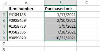
To get started, open the Excel spreadsheet that contains the dates you want to reformat. Select the cells that hold each date by clicking and dragging your mouse over them.

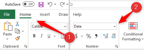
Once selected, click the down arrow to the right of the text box in the Number group of the Home tab.

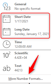
A drop-down menu will appear. There are two date format options to choose from in this menu: Short Date (1/17/2021) and Long Date (Sunday, January 17, 2021). You can select either of those or, if that’s not the format you’re looking for, click “More Number Formats” at the bottom of the menu. This opens the Format Cells window. You can also press Ctrl+1 (Command+1 on Mac) to open this window.

You’ll now be in the Date category of the Format Cells window. In the Type group, select the format you would like to use. If you prefer to choose a date format based on how a certain language and region formats dates, you can select an option from the Locale drop-down menu.

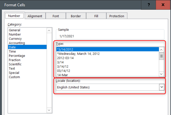
Click “OK” at the bottom of the window when you’ve selected the format you want to use. The dates in the previously selected cells will change to the new format.

Related: How to Add or Subtract Dates in Microsoft Excel

Take advantage of PREMIUM features.
Create your texts / logos without any limitation.
No attribution required when downloading.
No advertising on the website.
TextStudio.com PREMIUM - Monthly Membership

Create and Use Your Own Custom Date Format

There are plenty of different formats to choose from, but you can also make your own custom date format if you want. To do so, select the cells that contain the dates you want to format by clicking and dragging your cursor over them.

PearlMountain Image Converter

Next, press Ctrl+1 (Command+1 on Mac) to open the Format Cells window. You’ll automatically be in the Date category. Click “Custom” at the bottom of the Category list.

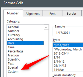
Next, you’ll notice a code in the Type text box.

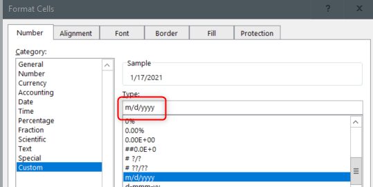
You can edit this code to create your own custom format. Each letter or letters in the code represents a display type. Here’s what each letter or letters mean:

So if you were to enter

    `m/d/yy`

in the Type box and then click “OK,” the dates in the selected cells would be formatted as:

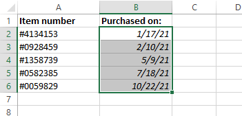
Play around with the different code combinations to find the perfect format that works for your spreadsheet.

When changing the date format, consider who’s going to be looking at the spreadsheet. If your spreadsheet contains a large amount of data, and you want to look at the data over a period of time, you can sort the data by date , regardless of the format being used.

Related: How to Sort by Date in Microsoft Excel