Mastering Precision: Tips & Techniques for Rounding Decimals in Microsoft Excel

Quick Links

• Round Off Decimal Values Using the ROUND Function
• Round Numbers Up or Down Using the ROUNDUP or ROUNDDOWN Functions

If you don’t want to show decimal values in Excel, you can simplify your numerical data using the ROUND functions. Excel offers three functions: ROUND, ROUNDUP, and ROUNDDOWN. Let’s take a look at how they work.

Using the ROUND functions in Excel is different than changing the number’s format. When you change how a number is formatted, you’re just changing how it looks in your workbook. When you change a number using the ROUND functions, you’re changing how it looks and how it’s stored.

The ROUND function rounds numbers to a specified number of decimal places. It rounds a number down if the digit in the next decimal place to the right is between zero and four, and it rounds up if that digit is five to nine. And as you might expect, the ROUNDUP function always rounds up and the ROUNDDOWN function always rounds down.

Round Off Decimal Values Using the ROUND Function

The ROUND function rounds numbers to a certain number of decimal places that you configure. If the next digit to the right is between zero and four, it rounds down. So, for example, if you were rounding down to two decimal places, 8.532 would become 8.53. If the next digit is between five and nine, it rounds up. So, 8.538 would become 8.54. The ROUND function can round numbers to the right or left of the decimal point.

You can apply the format to empty cells or to cells that already have numbers in them. You can also use ROUND as part of a more complicated formula if you want to. For example, you could create a formula that adds two columns together using the SUM function, and then rounds the result.

For this example, we’ve got a column of numbers named “Values” that contains our raw numbers. We’re creating a second column named “Results” that we’re going to use to round down the numbers in the “Values” column to three digits.

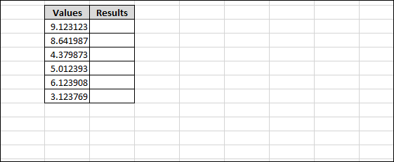
Select the cell where you want your rounded results to go.

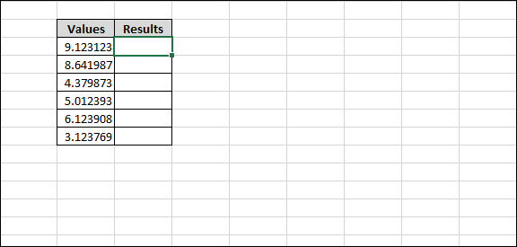
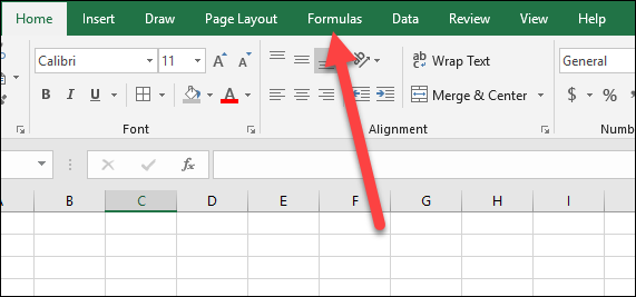
Navigate to the “Formulas” menu on the main ribbon.

Click the “Math & Trig” formulas drop-down menu.

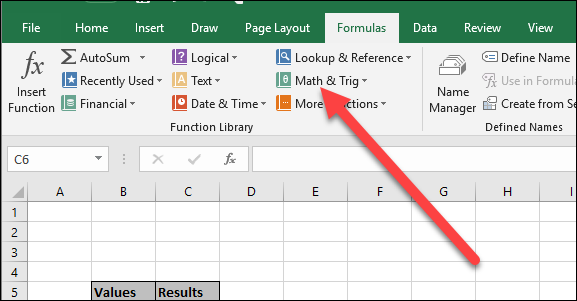
On the “Math & Trig” drop-down menu, click the “ROUND” function.

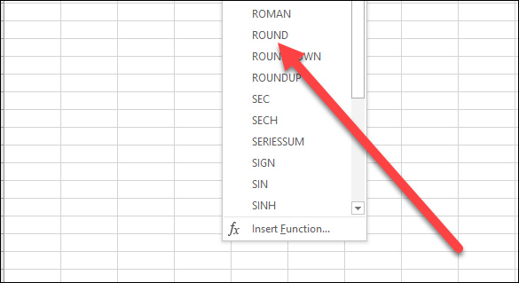
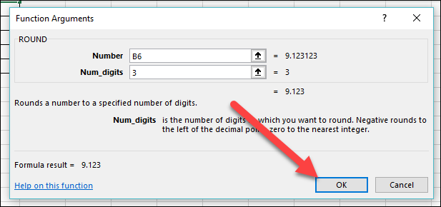
This pops up the Function Arguments window with the fields you’ll use for setting the ROUND function.

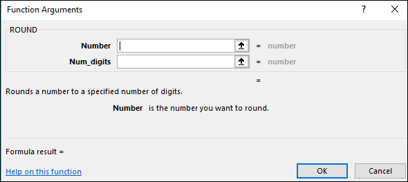
Use the “Number” field for the number you want to round. You can use type a straight up number in this field to round it, but more often you’ll want to call a number from an existing cell in your sheet. Here, we’re using B6 to specify the top cell in our “Values” column.

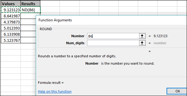
Use the “Num_Digits” field to specify how many digits the resulting number should have. You have some choices here:

• Positive Integer: Use a positive integer (such as 1, 2, and so on) to specify the number of digits after the decimal place to which you want to round. For example, entering “3” would round to three places after the decimal point.
• Zero: Enter “0” to round to the nearest integer.
• Negative Integer: Use a negative integer (such as -1, -2, and so on) to round to left of the decimal place. For example, if you were rounding the number 328.25 and input “-1” here, it would round you number to 330.

In our example, we’re inputting “3” so that it will round our result to three places after the decimal point.

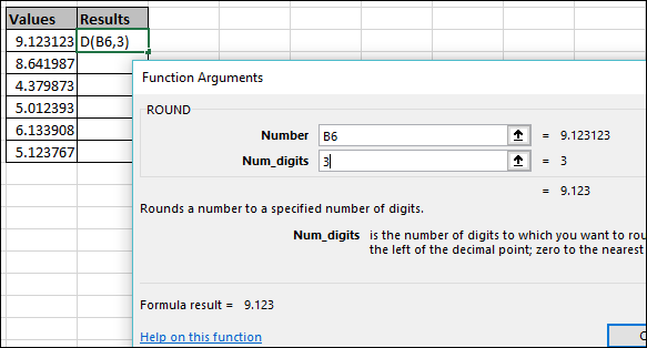
When you’re done, click the “OK” button.

And as you can see, our number is now rounded in the Results column.

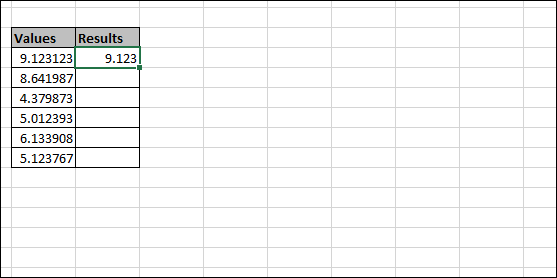
You can easily apply this formula to the rest of the numbers in your set by first clicking on the bottom right corner of the cell.

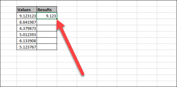
And then dragging to select the rest of the rows that you want to round.

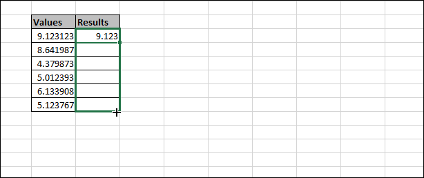
All of your values will now be rounded using the same properties you selected. You can also copy the cell to which you’ve already applied rounding, and then paste to other cells to copy the formula there.

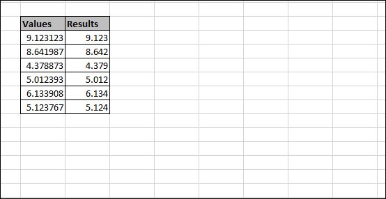
You can also do all this just using Excel’s Function bar if you want.

Select the column where you want your rounded numbers to go.

Click the Function bar to activate it.

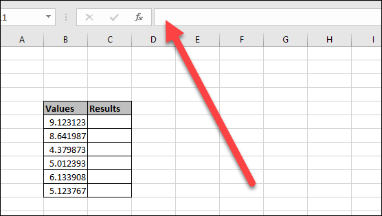
Type in your formula using the syntax:

=ROUND(number,num_digits)

Where “number” is the cell you want to round and “num_digits” identifies the number of digits to which you want to round.

For example, here’s how we’d type the same rounding formula we previously applied using the dialog box.

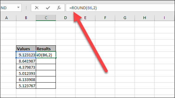
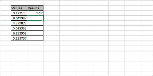
Hit Enter (or Return) after typing your formula, and your number is now rounded.

Round Numbers Up or Down Using the ROUNDUP or ROUNDDOWN Functions

Sometimes, you may want your numbers to just round numbers up or down instead of having the next digit decide that for you. That’s what the ROUNDUP and ROUNDDOWN functions are for, and and using them is pretty much identical to using the ROUND function.

Click the cell where you want your rounded result to go.

Head to Formulas > Math & Trig, and then choose either the “ROUNDUP” or “ROUNDDOWN” function from the dropdown menu.

WonderFox DVD Ripper Pro

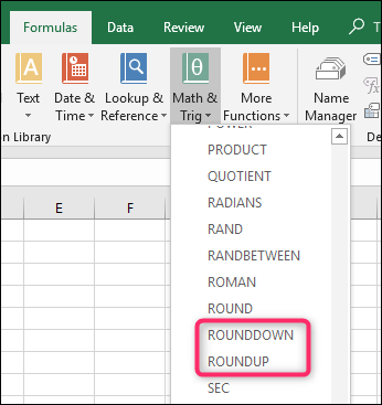
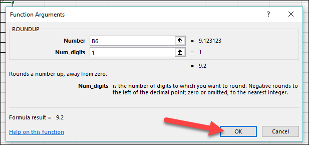
Enter the number (or cell) you want to round in the “Number” field. Enter the number of digits to which you want to round in the “Num_digits” field. And the same rules apply as with the ROUND function. A positive integer rounds to the right of the decimal point, zero rounds to the nearest integer, and a negative integer rounds to the left of the decimal point.

Click “OK” when you’ve got things set up.

And just like with the ROUND function, you can also set up the ROUNDUP and ROUNDDOWN functions by typing them into the Function bar, and you can use them as parts of a larger formula.