Essential 12 Spreadsheet Commands: A Must-Know Guide for All Excel Users

Quick Links

Microsoft Excel contains many functions that allow you to perform tasks without a calculator or extra work. But if you’re unfamiliar with formulas, it can feel intimidating. Here, we’ve listed 12 simple but useful Excel functions to get you started.

1. Add Numbers in Cells: SUM

One of the most basic things you can do with numbers is add them. Using the SUM function in Excel you can add numbers in cells.

The syntax is

    `SUM(value1, value2,...)`

where value1 is required and value2 is optional. So for each argument, you can use a number, cell reference, or cell range.

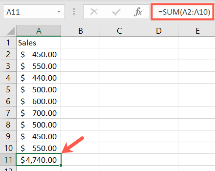
For example, to add the numbers in cells A2 through A10, you would enter the following and press Enter:

=SUM(A2:A10)

You then get your result in the cell containing the formula.

2. Average Numbers in Cells: AVERAGE

Averaging a group of numbers is another common mathematical function.

The syntax is the same for the AVERAGE function in Excel as with the SUM function, AVERAGE(value1, value2,...) with value1 required and value2 optional. You can enter cell references or ranges for the arguments.

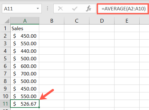
To average the numbers in cells A2 through A10, you would enter the following formula and press Enter:

=AVERAGE(A2:A10)

You then get your average in the cell containing the formula.

3. Find the High or Low Value: MIN and MAX

When you need to find the minimum or maximum value in a range of cells, you use the MIN and MAX functions.

The syntaxes for these functions are the same as the others, MIN(value1, value2,...) and MAX(value1, value2,...) with value1 required and value2 optional.

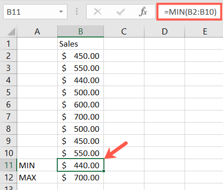
To find the minimum, lowest value, in a group of cells, enter the following replacing the cell references with your own. Then, hit Enter:

=MIN(B2:B10)

And to find the maximum, highest value, use:

=MAX(B2:B10)

You’ll then see the smallest or largest value in the cell with the formula.

4. Find the Middle Value: MEDIAN

Instead of the minimum or maximum value, you may want the middle one.

As you may have guessed, the syntax is the same, MEDIAN(value1, value2,...) with the first argument required and the second optional.

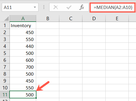
For the middle value in a range of cells enter the following and press Enter:

=MEDIAN(A2:A10)

You’ll then see the middle number of your cell range.

5. Count Cells Containing Numbers: COUNT

Maybe you’d like to count how many cells in a range contain numbers. For this, you would use the COUNT function.

The syntax is the same as the above two functions, COUNT(value1, value2,...) with the first argument required and the second optional.

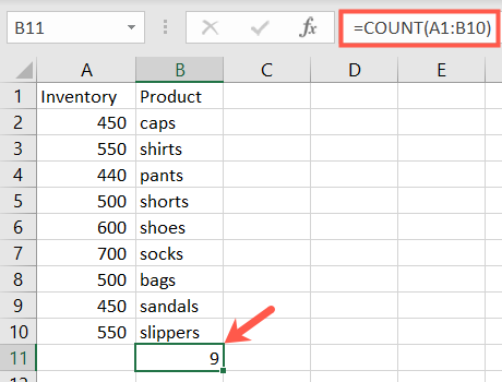
To count the number of cells that contain numbers in the range A1 through B10, you would enter the following and press Enter:

=COUNT(A1:B10)

You then get your count in the cell containing the formula.

Epubor Ultimate for Win：Helps you read books anywhere, including the best eBook Converter + eBook DRM Removal functions.

6. Insert the Current Date and Time: NOW

If you’d like to display the current date and time whenever you open your spreadsheet, use the NOW function in Excel.

The syntax is NOW() because the function has no required arguments. You can, however, add or remove from the current date and time if you like.

To return the current date and time, enter the following and press Enter:

=NOW()

To return the date and time five days in the future from the current date and time, enter this formula and hit Enter:

=NOW()+5

And here’s how the results would look for each of the above formulas.

Forex Robotron Gold Package

7. Round to a Certain Number of Digits: ROUND

If you have decimal numbers in your sheet that you want to round up or down, use the ROUND function in Excel.

The syntax is ROUND(value1, digits) where both arguments are required. For value1 , use the number you want to round. For digits , use the number of decimal places to round the number.

For example, to round the number 2.25 up one decimal place, enter the following and press Enter:

=ROUND(2.25,1)

And you have your results. If you want to round down, simply use a negative number for the digits argument.

8. Truncate a Number by Removing the Fraction: TRUNC

Maybe you’d prefer to truncate a number rather than round it. Using the TRUNC function , you can remove the fraction from the number.

The syntax is TRUNC(value1, digits) with value1 required and digits optional. If you don’t enter the digits, the default value is zero.

So, to truncate the number 7.2 you would enter the following and press Enter:

=TRUNC(7.2)

The result of this formula would be the number seven.

Take advantage of PREMIUM features.
Create your texts / logos without any limitation.
No attribution required when downloading.
No advertising on the website.
TextStudio.com PREMIUM - Monthly Membership

Screensaver Factory, Create stunning professional screensavers within minutes. Create screensavers for yourself, for marketing or unlimited royalty-free commercial distribution. Make screensavers from images, video and swf flash, add background music and smooth sprite and transition effects. Screensaver Factory is very easy to use, and it enables you to make self-installing screensaver files and CDs for easy setup and distribution. Screensaver Factory is the most advanced software of its kind.

9. Find the Product by Multiplying Cells: PRODUCT

If you need to multiply several cells , using the PRODUCT function is more efficient than using the multiplication symbol (*) in a formula.

The syntax is PRODUCT(value1, value2,...) with value1 required and value2 optional. You can use value1 for the cell range and value2 for an additional cell range if needed.

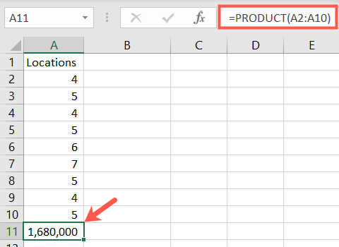
To find the product of cells A2 through A10, you would enter the following and hit Enter:

=PRODUCT(A2:A10)

As you can see, this is much simpler than entering A2 * A3 * A4 , and so on.

10. Use the Reference Number of a Given Cell: COLUMN and ROW

With the COLUMN and ROW functions in Excel, you can return the position number of a cell. These functions are useful for entering a series of reference numbers in your sheet, or row numbers , for instance.

The syntax for each is COLUMN(reference) and ROW(reference) where the argument is not required. If you don’t enter an argument, the formula returns the reference for the cell containing the formula.

For example, if you enter the following formula into cell B2, the result would be 2 because B2 is in the second row.

=ROW()

But if you enter the following formula with an argument, you’ll receive the reference number for the cell.

=ROW(C5)

You can see here; the result is 5 because C5 is in the fifth row.

Forex Robotron Basic Package

11. Eliminate White Space: TRIM

Oftentimes you when you paste or import data, it contains extra spaces. The TRIM function eliminates white space.

The syntax is TRIM(reference) with the argument required for the cell reference containing the data.

To remove extra spaces from cell A1, you would enter the following and hit Enter:

=TRIM(A1)

You’ll then see the data in your referenced cell without the leading and trailing spaces.

12. Count the Number of Characters in a String: LEN

Maybe you need to find the number of characters in a string of text. Here, you’d use the LEN function in Excel.

The syntax is LEN(reference) with the argument required for the cell reference containing the text.

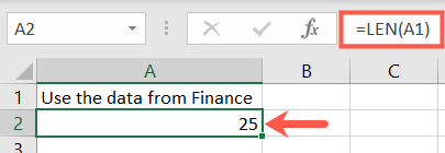
To find the number of characters in cell A1, enter the following formula and press Enter:

=LEN(A1)

The result is 25 because “Use the data from Finance” contains that number of characters and note that spaces are counted as characters.

PaperScan Professional： PaperScan Scanner Software is a powerful TWAIN & WIA scanning application centered on one idea: making document acquisition an unparalleled easy task for anyone.

There are many other useful functions in Excel such as VLOOKUP for finding a value and CONCATENATE for joining strings of text . But this list of the basics should help you with simple tasks while becoming more familiar with using functions.

Win Answers

Essential 12 Spreadsheet Commands: A Must-Know Guide for All Excel Users