Efficient Z-Score Computation Techniques with Microsoft Excel Explained

Quick Links

• What is a Z-Score and what do the AVERAGE, STDEV.S, and STDEV.P functions do?
• Let’s Look at an Example
• Calculating the Z-Score without using ‘Helper’ Cells

A Z-Score is a statistical value that tells you how many standard deviations a particular value happens to be from the mean of the entire data set. You can use AVERAGE and STDEV.S or STDEV.P formulas to calculate the mean and standard deviation of your data and then use those results to determine the Z-Score of each value.

What is a Z-Score and what do the AVERAGE, STDEV.S, and STDEV.P functions do?

A Z-Score is a simple way of comparing values from two different data sets. It is defined as the number of standard deviations away from the mean a data point lies. The general formula looks like this:

=(DataPoint-AVERAGE(DataSet))/STDEV(DataSet)

Here’s an example to help clarify. Say you wanted to compare the test results of two Algebra students taught by different teachers. You know the first student got a 95% on the final exam in one class, and the student in the other class scored 87%.

At first glance, the 95% grade is more impressive, but what if the teacher of the second class gave a more difficult exam? You could calculate the Z-Score of each student’s score based on the average scores in each class and the standard deviation of the scores in each class. Comparing the Z-Scores of the two students could reveal that the student with the 87% score did better in comparison to the rest of their class than the student with the 98% score did in comparison to the rest of their class.

The first statistical value you need is the ‘mean’ and Excel’s “AVERAGE” function calculates that value. It simply adds up all of the values in a cell range and divides that sum by the number of cells containing numerical values (it ignores blank cells).

The other statistical value we need is the ‘standard deviation’ and Excel has two different functions to calculate the standard deviation in slightly different ways.

Previous versions of Excel only had the “STDEV” function, which calculates the standard deviation while treating the data as a ‘sample’ of a population. Excel 2010 broke that into two functions that calculate the standard deviation:

• STDEV.S: This function is identical to the previous “STDEV” function. It calculates the standard deviation while treating the data as a ‘sample’ of a population. A sample of a population might be something like the particular mosquitoes collected for a research project or cars that were set aside and used for crash safety testing.
• STDEV.P: This function calculates the standard deviation while treating the data as the entire population. An entire population would be something like all mosquitoes on Earth or every car in a production run of a specific model.

Which you choose is based on your data set. The difference will usually be small, but the result of the “STDEV.P” function will always be smaller than the result of the “STDEV.S” function for the same data set. It is a more conservative approach to assume there is more variability in the data.

Let’s Look at an Example

For our example, we have two columns (“Values” and “Z-Score”)and three “helper” cells for storing the results of the “AVERAGE,” “STDEV.S,” and “STDEV.P” functions. The “Values” column contains ten random numbers centered around 500, and the “Z-Score” column is where we will calculate the Z-Score using the results stored in the ‘helper’ cells.

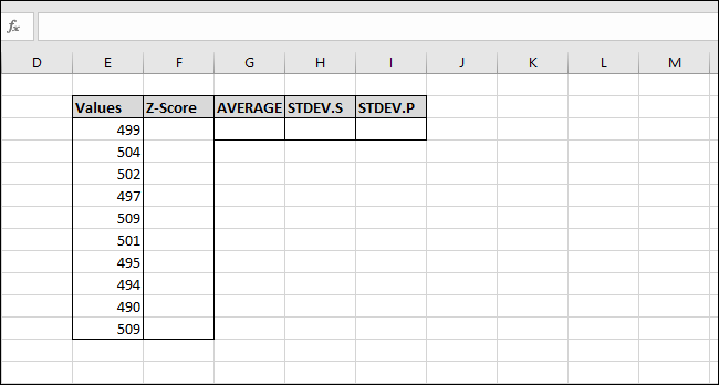
First, we will calculate the mean of the values using the “AVERAGE” function. Select the cell where you will store the result of the “AVERAGE” function.

Epubor Audible Converter for Win： Download and convert Audible AAXC/AA/AAX to MP3 with 100% original quality preserved.

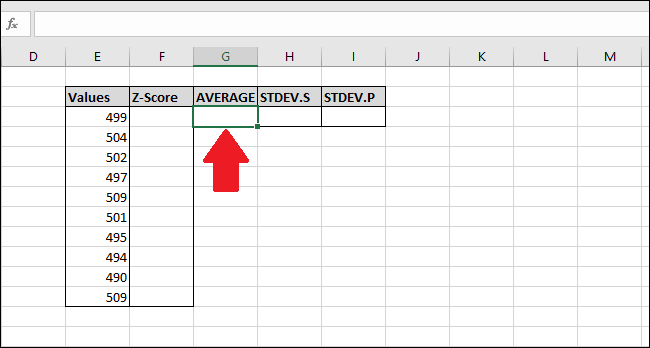
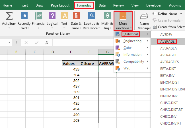
Type in the following formula and press enter -or- use the “Formulas” menu.

=AVERAGE(E2:E13)

To access the function through the “Formulas” menu, select the “More Functions” drop-down, select the “Statistical” option, and then click on “AVERAGE.”

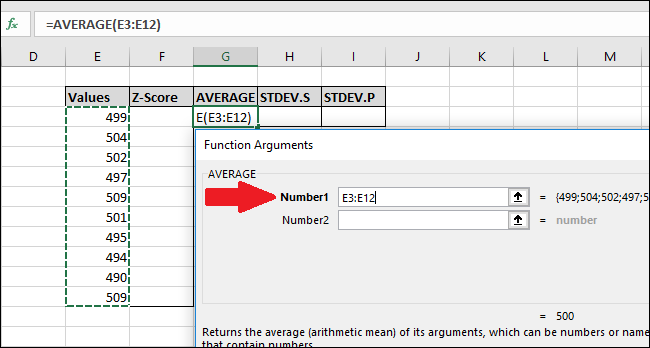
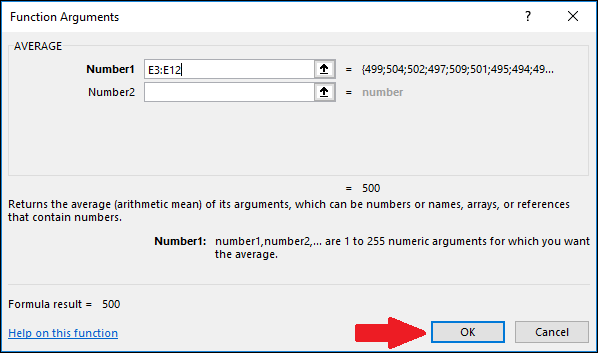
In the Function Arguments window, select all of the cells in the “Values” column as the input for the “Number1” field. You don’t need to worry about the “Number2” field.

Now press “OK.”

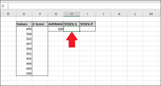
Next, we need to calculate the standard deviation of the values using either the “STDEV.S” or “STDEV.P” function. In this example, we will show you how to calculate both values, starting with “STDEV.S.” Select the cell where the result will be stored.

To calculate the standard deviation using the “STDEV.S” function, type in this formula and press Enter (or access it through the “Formulas” menu).

=STDEV.S(E3:E12)

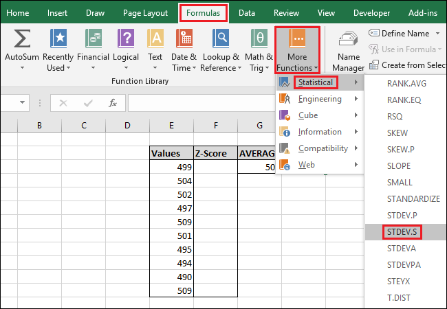
To access the function through the “Formulas” menu, select the “More Functions” drop-down, select the “Statistical” option, scroll down a bit, and then click the “STDEV.S” command.

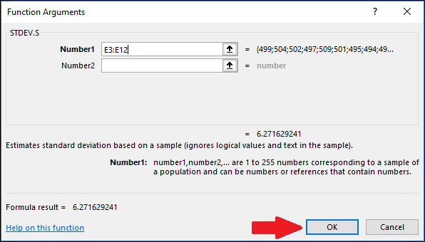
In the Function Arguments window, select all of the cells in the “Values” column as the input for the “Number1” field. You don’t need to worry about the “Number2” field here, either.

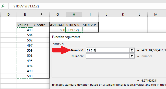
Now press “OK.”

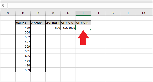
Next, we will calculate the standard deviation using the “STDEV.P” function. Select the cell where the result will be stored.

To calculate the standard deviation using the “STDEV.P” function, type in this formula and press Enter (or access it through the “Formulas” menu).

=STDEV.P(E3:E12)

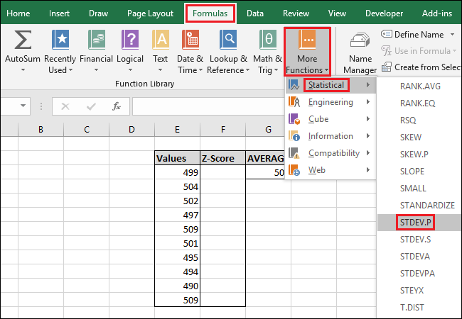
To access the function through the “Formulas” menu, select the “More Functions” drop-down, select the “Statistical” option, scroll down a bit, and then click the “STDEV.P” formula.

EaseText Audio to Text Converter for Windows (Personal Edition) - An intelligent tool to transcribe & convert audio to text freely

In the Function Arguments window, select all of the cells in the “Values” column as the input for the “Number1” field. Again, you won’t need to worry about the “Number2” field.

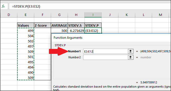
Now press “OK.”

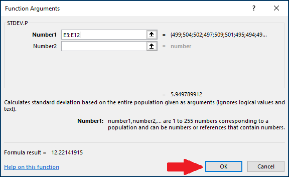
Now that we have calculated the mean and standard deviation of our data, we have all we need to calculate the Z-Score. We can use a simple formula that references the cells containing the results of the “AVERAGE” and “STDEV.S” or “STDEV.P” functions.

Select the first cell in the “Z-Score” column. We will use the result of the “STDEV.S” function for this example, but you could also use the result from “STDEV.P.”

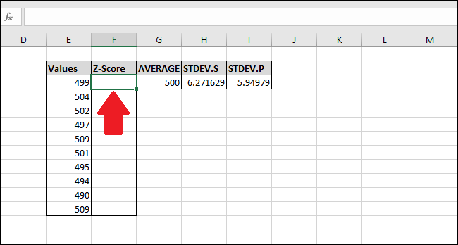
Type in the following formula and hit Enter:

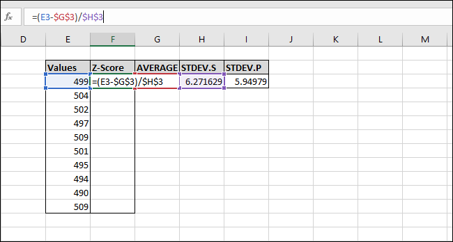
=(E3-$G$3)/$H$3

Alternatively, you could use the following steps to enter the formula instead of typing:

1. Click cell F3 and type =(
2. Select cell E3. (You can press the left-arrow-key once or use the mouse)
3. Type the minus sign -
4. Select cell G3 then press F4 to add the “$” characters to make an ‘absolute’ reference to the cell (it will cycle through “G3” > “**$G$3” > “G$3” > “$**G3” > “G3” if you continue pressing F4)
5. Type )/
6. Select cell H3 (or I3 if you are using “STDEV.P”) and press F4 to add the two “$” characters.
7. Press Enter

The Z-Score has been calculated for the first value. It is 0.15945 standard deviations below the mean. To check the results, you can multiply the standard deviation by this result (6.271629 * -0.15945) and check that the result is equal to the difference between the value and the mean (499-500). Both results are equal, so the value makes sense.

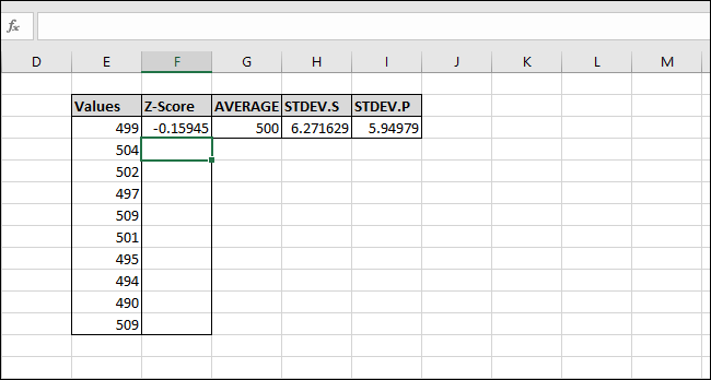
Let’s calculate the Z-Scores of the rest of the values. Highlight the whole ‘Z-Score’ column starting with the cell containing the formula.

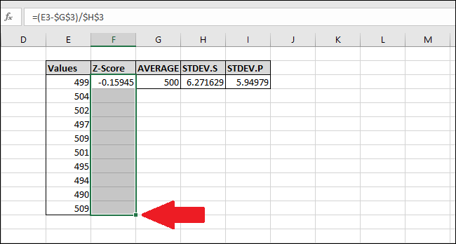
Press Ctrl+D, which copies the formula in the top cell down through all the other selected cells.

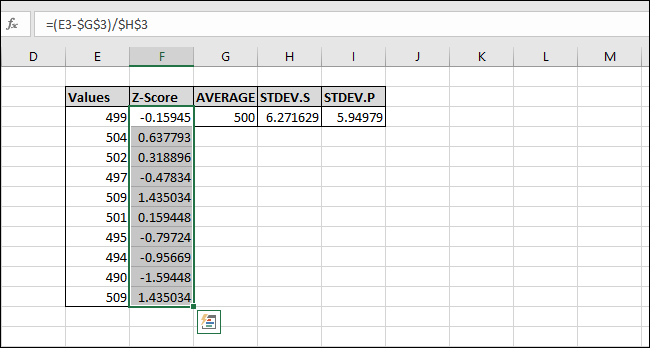
Now the formula has been ‘filled-down’ to all of the cells, and each will always reference the correct “AVERAGE” and “STDEV.S” or “STDEV.P” cells because of the “$” characters. If you get errors, go back and make sure the “$” characters are included in the formula you entered.

WPS Office Premium ( File Recovery, Photo Scanning, Convert PDF)–Yearly

Calculating the Z-Score without using ‘Helper’ Cells

Helper cells store a result, like the ones storing the results of the “AVERAGE,” “STDEV.S,” and “STDEV.P” functions. They can be useful but aren’t always necessary. You can skip them altogether when calculating a Z-Score by using the following generalized formulas, instead.

Here’s one using the “STDEV.S” function:

=(Value-AVERAGE(Values))/STDEV.S(Values)

And one using the “STEV.P” function:

=(Value-AVERAGE(Values))/STDEV.P(Values)

When entering the cell ranges for the “Values” in the functions, be sure to add absolute references (“$” using F4) so that when you ‘fill-down’ you aren’t calculating the average or standard deviation of a different range of cells in every formula.

If you have a large data set, it may be more efficient to use helper cells because it doesn’t calculate the result of the “AVERAGE” and “STDEV.S” or “STDEV.P” functions each time, saving processor resources and speeding up the time it takes to calculate the results.

Also, “$G$3” takes fewer bytes to store and less RAM to load than “AVERAGE($E$3:$E$12).”. This is important because the standard 32-bit version of Excel is limited to 2GB of RAM (the 64-bit version does not have any limitations on how much RAM can be used).