Easy Steps to Generate Basic Invoices in Microsoft Excel

Quick Links

• Using an Invoice Template
• Creating a Simple Invoice in Excel from Scratch

Whether you’re a freelancer doing work for multiple companies, or a business that plans on extending a credit line to its customers, you’re going to need an invoice. Creating a custom invoice in Excel isn’t difficult. You’ll be ready to submit your invoice and receive payments in no time.

Using an Invoice Template

Creating a simple invoice in Excel is relatively straightforward. Create a few tables, set a few rules, add a bit of information, and you’re good to go. Alternatively, there are many websites out there that provide free invoice templates created by actual accountants. You can use these instead, or even download one to use as inspiration for when you’re making your own.

Excel also provides its own library of invoice templates you can use. To access these templates, open Excel and click the “File” tab.

Here, select “New” and type “Invoice” into the search bar.

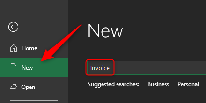
Press Enter and a collection of invoice templates will appear.

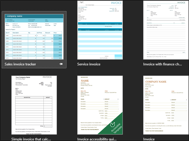
Browse through the available templates to find one you like.

Creating a Simple Invoice in Excel from Scratch

To make a simple invoice in Excel, we need first to understand what information is required. To keep it simple, we’ll create an invoice using only the information necessary to receive payment. Here’s what we need:

• Seller Information
  • Name
  • Address
  • Phone Number
• Buyer Information
  • Company Name
  • Address
• Date of Invoice
• Invoice Number
• Item Description (of service or product sold)
• Item Price (of individual product or service)
• Total Amount Due
• Method of Payment

Let’s get started.

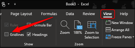
First, open up a blank Excel sheet. The first thing we’re going to want to do is to get rid of the gridlines, giving us a clean excel sheet to work in. To do so, head over to the “View” tab and uncheck “Gridlines” in the “Show” section.

Now let’s resize some of the columns and rows. This will give us extra room for some of the lengthier information like item descriptions. To resize a row or column, click and drag.

By default, rows are set to a height of 20 pixels and columns are set at a width of 64 pixels. Here’s how we recommend setting your rows and columns to have an optimized setup.

Rows:

• Row 1: 45 pixels

Columns:

• Column A: 385 pixels
• Column B: 175 pixels
• Column C: 125 pixels

Row 1 will have your name and the word “Invoice.” We want that information to be immediately apparent to the recipient, so we give a little extra space to increase the font size of this information to ensure it grabs the recipient’s attention.

Column A contains the majority of important (and potentially lengthy) information in the invoice. This includes buyer and seller information, item description, and method of payment. Column B contains the specific dates of the items listed, so it doesn’t require as much space. Finally, column C will include the invoice number, invoice date, the individual price of each item listed, and the total amount due. This information is also short in length, so it doesn’t require much room.

Go ahead and adjust your rows and cells to the suggested specifications, and let’s get started with plugging in our information!

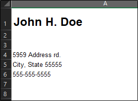
In column A, row 1, go ahead and enter your name. Give it a larger font size (Around 18pt font) and bold the text so that it stands out.

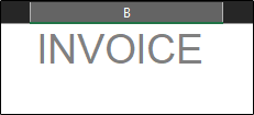
In column B, row 1, type “Invoice” to make it immediately clear what the document is. We recommend a 28pt font using all caps. Feel free to give it a lighter color if you’d like.

In Column A, Rows 4, 5, and 6, we will input our address and phone number.

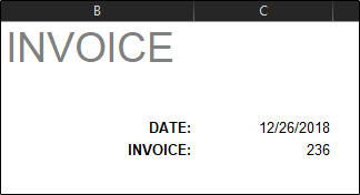
In column B, rows 4 and 5, type “DATE:” and “INVOICE:” with bold text and align the text to the right. Column C rows 4 and 5 is where you’ll enter the actual date and invoice number.

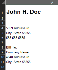
Finally, for the last part of the basic information, we’ll enter the text “Bill To:” (in bold) in column A, row 8. Below that in rows 9, 10, and 11, we’ll enter the recipient information.

Now we need to make a table to list our items, fulfillment dates, and specific amounts. Here’s how we’ll set it up:

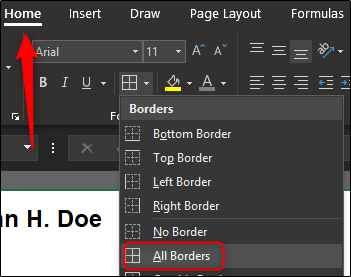
First, we’ll merge column A and B in row 14. This will act as the header for our listed items (column A, rows 15-30) and our fulfillment dates (column B, rows 15-30). After you’ve merged column A and B in row 14, give the cell a border. You can do so by going to the “Font” section of the “Home” tab, selecting the border icon, and choosing your desired border type. For now, we’ll use “All Borders.”

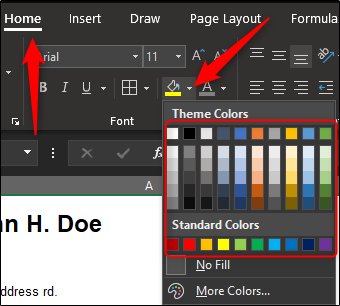
Do the same for cell C14. Feel free to shade your cells if you like. We’ll do a light gray. To fill your cells with a color, select the cells, select the arrow next to the “Fill Color” icon in the “Font section of the “Home” tab, and select your color from the drop-down menu.

EmEditor Professional (Lifetime License, non-store app)

In the first highlighted cell, type “DESCRIPTION” and align the text in the center. For C14, type “AMOUNT” with center alignment. Bold the text for both. Now you’ll have your table header.

We want to make sure we have a table big enough to list all of our items. In this example, we’ll use sixteen rows. Give or take as many as you need.

Go to the bottom of where your table will be and give the first two cells in the row a bottom border.

Now highlight cells C15-29 and give them all left and right borders.

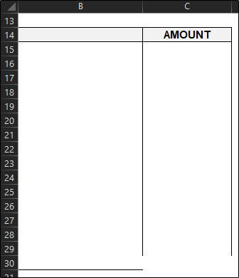
Now, select cell C30 and give it left, right, and bottom borders. Finally, we’ll add a “Total Sum” section on our table. Highlight cell C31 and give it borders around the entire cell. You may also give it a shade of color so that it stands out. Be sure to label it with “TOTAL” in the cell next to it.

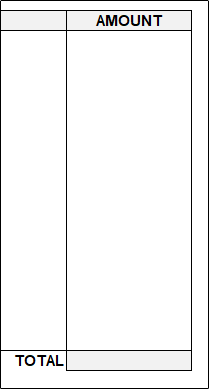
That completes the frame of our table. Now let’s set some rules and add a formula to wrap it up.

We know our fulfillment dates will be in column B, rows 15-30. Go ahead and select those cells. Once all of them are selected, click the “Format Number” box in the “Number” section of the “Home” tab.

OtsAV DJ Pro

Once selected, a drop-down menu will appear. Select the “Short Date” option. Now if you enter a number such as 12/26 in any of those cells, it will automatically reformat it to the short date version.

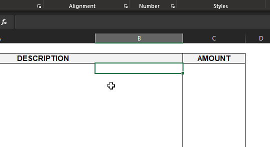
Similarly, if you highlight cells C15-30, which is where our item amount will go, and select the “Currency” option, then enter an amount in those cells, it will be reformatted to reflect that amount.

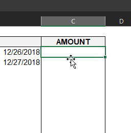
To automatically add all of the individual amounts and have it reflected in the “Sum” cell we created, select the cell (C31 in this example) and enter the following formula:

=SUM(C15:C30)

Now if you enter (or remove) any number in the individual amount cells, it will automatically reflect in the sum cell.

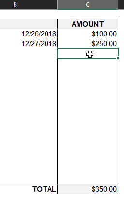
This will make things more efficient for you in the long run.

Moving on, enter the text “Method of Payment:” in A34.

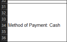
The information you put next to that is between you and the recipient. The most common forms of payment are cash, check, and wire. Sometimes you may be asked to accept a money order. Some companies even prefer to make a direct deposit or use PayPal.

Now for the finishing touch, don’t forget to thank your customer or client!

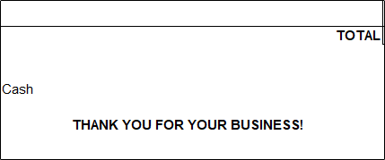
Start sending out your invoice and collecting your pay!